지난 글에서 Dijkstra's Algorithm(다익스트라, 데이크스트라 알고리즘)에 대해 알아봤습니다. 오늘은 Neo4j에서 실행해보도록 하겠습니다.
Unweighted 와 Weighted Shortest Path 이해하기.
최단거리 계산에는 크게 두가지 방법이 있습니다. 하나는 노드간 몇 회만 뛰어넘는지만 계산하는 방식, 다른 하나는 노드 사이의 실제 거리 값을 계산하는 방식이 있습니다. 우선 그림으로 둘의 차이를 간략히 설명하겠습니다.

앞으로 실행할 알고리즘은 위와 같습니다. 유럽의 여러 도시들과 그 사이의 거리를 표시한 것을 볼 수 있습니다. Neo4j 그래프에선 기본으로 화살표가 생겨 마치 한방향으로 가는것 같지만, 이는 프로그램 기본사항이므로 무시하도록 합시다.
Unweighted Shortest Path 계산해보기
얼마나 적은 Hop을 통해서 위치 점에 도달하는지
Unweighted는 노드 사이에있는 엣지의 cost값(여기서는 거리)을 무시하고, 노드 사이에 거치는 횟수만 신경쓰는 방법입니다. 그림이 간단하니 눈으로도 계산할수 있습니다.
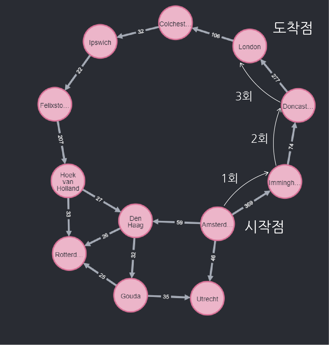
위와 같이 암스테르담에서 런던까지, 2개의 도시거치는 다시말해 3번 이동 하면 도달할 수 있는 것을 볼 수 있습니다.
코드로 실행하기
코드는 다음과 같습니다.
MATCH (source:Place {id: "Amsterdam"}),
 (destination:Place {id: "London"})
CALL gds.alpha.shortestPath.stream({
 startNode: source,
 endNode: destination,
 nodeProjection: "*",
 relationshipProjection: {
 all: {
 type: "*",
 orientation: "UNDIRECTED"
 }
 }
})
YIELD nodeId, cost
RETURN gds.util.asNode(nodeId).id AS place, cost;
기본적인 구조 이해
MATCH ~
CALL gds.alpha.shortestPath.stream(~)
YIELD nodeId, cost
RETURN gds.util.asNode(nodeId).id AS place, cost;
MATCH 이하 구문은, 변수를 할당하는 부분이라고 보면 됩니다.
CALL 이하 부분은 gds 라이브러리를 사용할때 쓰는 방법으로, stream 으로 쓰면 중간 결과를 보여주고, write라고 쓰면 최종 결과만 보여줍니다. ~에는 원하는 query 방법을 매핑합니다.
한줄한줄 해석해보도록 하겠습니다.
MATCH (source:Place {id: "Amsterdam"}),
 (destination:Place {id: "London"})
Place 노드 중, id가 암스테르담이면 source에, 런던이면 destination에 할당 합니다.
CALL gds.alpha.shortestPath.stream({
 startNode: source,
 endNode: destination,
 nodeProjection: "*",
 relationshipProjection: {
 all: {
 type: "*",
 orientation: "UNDIRECTED"
 }
 }
})
위에서 할당한
source를 startNode
destination을 endNode
nodeProjection 은 어떤 노드들을 사용할지 여기서는 모든 노들를 사용하는 의미에서 "*", 특정 범주의 노드만 사용하고 싶다면 "범주이름"
relationshipProjection은 어떤 edge를 사용할지 정의. 여기선 모든 엣지를 사용하며, 방향은 무시1.
더 자세한 문법을 알고싶으시다면 맨 아래 링크를 참조해주시길 바랍니다. 그럼 실행해보도록 하겠습니다.
실행
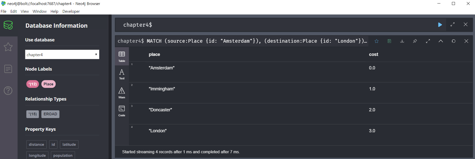
기본 문법으론 다음과 같이 몇번 건너 뛰었는지 나오게 됩니다. 하지만 우리는 실제 거리값을 구하고 싶죠.
거리값을 표시해주는 코드로 실행
MATCH (source:Place {id: "Amsterdam"}),
 (destination:Place {id: "London"})
CALL gds.alpha.shortestPath.stream({
 startNode: source,
 endNode: destination,
 nodeProjection: "*",
 relationshipProjection: {
 all: {
 type: "*",
 orientation: "UNDIRECTED"
 }
 }
})
YIELD nodeId, cost
WITH collect(gds.util.asNode(nodeId)) AS path
UNWIND range(0, size(path)-1) AS index
WITH path[index] AS current, path[index+1] AS next
WITH current, next, [(current)-[r:EROAD]-(next) | r.distance][0] AS distance
WITH collect({current: current, next:next, distance: distance}) AS stops
UNWIND range(0, size(stops)-1) AS index
WITH stops[index] AS location, stops, index
RETURN location.current.id AS place,
 reduce(acc=0.0,
 distance in [stop in stops[0..index] | stop.distance] |
 acc + distance) AS cost;
YIELD위의 코드는 동일한 것을 볼 수 있습니다. WITH 이하 부분은 루프로 보입니다.
보이는대로 해석해보겠습니다.
WITH collect() AS path -> collect 괄호 안의 내용을 path라는 list로 정의한다
UNWIND range() AS index -> 이 range의 각 값을 index로 정의한다. 즉 Main loop의 시작
WITH path[index] AS current, path[index+1] AS next -> 현재 index에 해당하는 path(node)는 current로, 그 다음은 next로 할당한다.
WITH current, next, [(current)-[r:EROAD]-(next) | r.distance][0] AS distance -> current와 next 사이의 relation(edge)의 0번 값을 distance로 정의한다.
WITH collect({current: current, next:next, distance: distance}) AS stops -> 위에서 정의 했던 값들로 stops라는 list를 정의한다.
UNWIND range(0, size(stops)-1) AS index -> stops의 index를 정의한다. Main loop 실행
WITH stops[index] AS location, stops, index -> index에 해당하는 stops는 location으로 할당하고 stops, index도 사용한다.
RETURN location.current.id AS place,
reduce(acc=0.0, distance in [stop in stops[0..index] | stop.distance] | acc + distance) AS cost;
-> location의 current의 id를 place로 return 하고, stops안의 stop에서 distance를 acc 에 더해 cost로 내보낸다.
실행
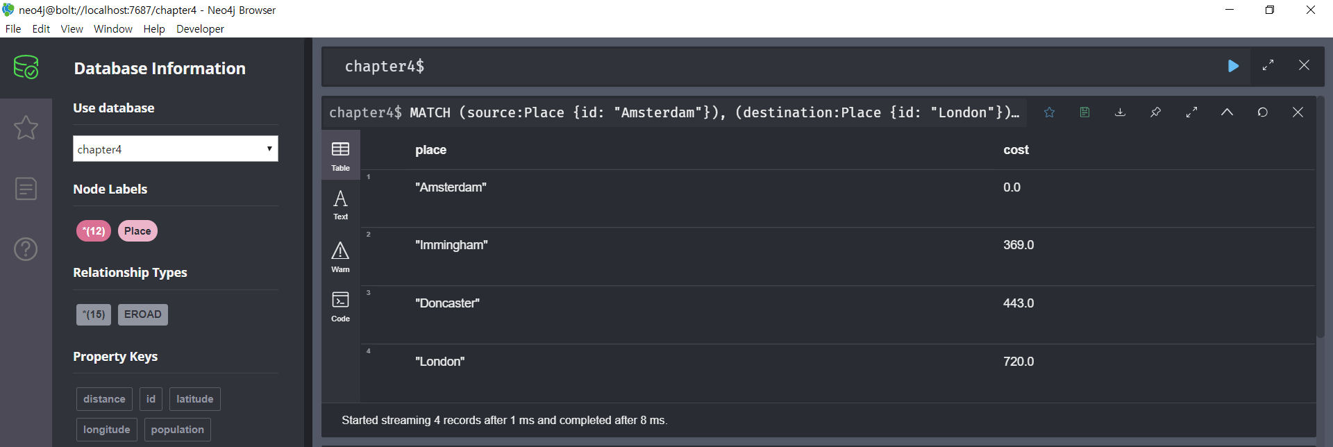
다음과 같이 실행되었습니다.
Weighted Shortest Path 계산해보기
얼마나 짧은 거리를 이동하는지
Weighted Shortest Path는 도시를 몇번 건너는지를 따지지 않습니다. 원하는 지점까지 얼마나 짧게 갈 수 있는지만 계산합니다.
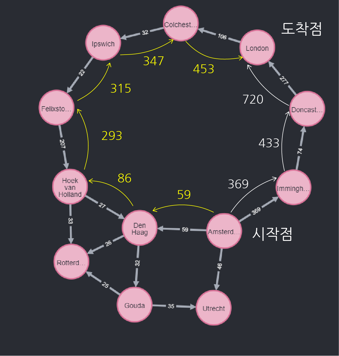
위의 그림에서 볼 수 있듯이, Unweighted에서는 몇번 건너뛰었는지만 신경씁니다. 따라서 3번만에 도달할수 있는 흰색 루트를 선택하게 됩니다. 반면 Weighted에서는 거리가 최단이 되는 루트를 찾는것을 볼 수 있습니다.
코드로 실행해보기
MATCH (source:Place {id: "Amsterdam"}),
 (destination:Place {id: "London"})
CALL gds.alpha.shortestPath.stream({
 startNode: source,
 endNode: destination,
 nodeProjection: "*",
 relationshipProjection: {
 all: {
 type: "*",
 properties: "distance",
 orientation: "UNDIRECTED"
 }
 },
 relationshipWeightProperty: "distance"
})
YIELD nodeId, cost
RETURN gds.util.asNode(nodeId).id AS place, cost;relationshipWeightProperty가 추가된 것을 볼 수 있습니다.
결과는 다음과 같습니다

끝맺으며
다음과 같은 질문들
- Cypher의 loop 구문을 알아봐야 겠다.
- gds를 쓰는 convention을 알아보자
- 테이블 대신 node로 나오게도 해봤는데, 조금 보기에 불편했다.
'아카이브 > 프로그래밍' 카테고리의 다른 글
| [그래프 데이터베이스][무작정해보기] [7/30] A*(A-star) Algorithm Neo4j에서 실행해보기 (0) | 2021.01.11 |
|---|---|
| [그래프 데이터베이스][무작정해보기] [6/30] A*(A-star) Algorithm 그림으로 이해하기. (0) | 2021.01.10 |
| [그래프 데이터베이스][무작정해보기] [4/30]Dijkstra's Algorithm(다익스트라, 데이크스트라 알고리즘) (0) | 2021.01.02 |
| [그래프 데이터베이스][무작정해보기] [3/30] 웹상의 CSV로 부터 Graph 생성하기 (1) | 2021.01.01 |
| [그래프 데이터베이스][무작정해보기] [2/30] 저장위치 설정 / 플러그인 설치 / 앞으로 다룰 알고리즘 (0) | 2020.12.30 |
![[그래프 데이터베이스][무작정해보기] [7/30] A*(A-star) Algorithm Neo4j에서 실행해보기](http://i1.daumcdn.net/thumb/C176x120.fwebp.q85/?fname=https%3A%2F%2Fblog.kakaocdn.net%2Fdna%2FdPM03e%2FbtqTcRwfLcU%2FAAAAAAAAAAAAAAAAAAAAAH5v8PDpzSTdapZYrxOzcWz3JG47EytiJtIl51uoNlg9%2Fimg.png%3Fcredential%3DyqXZFxpELC7KVnFOS48ylbz2pIh7yKj8%26expires%3D1774969199%26allow_ip%3D%26allow_referer%3D%26signature%3DHHsxkQpU8b4G2ggsOLfNubJuAOo%253D)
![[그래프 데이터베이스][무작정해보기] [6/30] A*(A-star) Algorithm 그림으로 이해하기.](http://i1.daumcdn.net/thumb/C176x120.fwebp.q85/?fname=https%3A%2F%2Fblog.kakaocdn.net%2Fdna%2FQxfiZ%2FbtqSZyc1Etr%2FAAAAAAAAAAAAAAAAAAAAAOpOvubQY5aOHUXchmFRPS4hqgKYYSHbxiiY8oEzgax5%2Fimg.png%3Fcredential%3DyqXZFxpELC7KVnFOS48ylbz2pIh7yKj8%26expires%3D1774969199%26allow_ip%3D%26allow_referer%3D%26signature%3DDnE7%252Fu4u2Pr5GWMQFs%252Fgm9hgHT4%253D)
![[그래프 데이터베이스][무작정해보기] [4/30]Dijkstra's Algorithm(다익스트라, 데이크스트라 알고리즘)](http://i1.daumcdn.net/thumb/C176x120.fwebp.q85/?fname=https%3A%2F%2Fblog.kakaocdn.net%2Fdna%2FcOPgBI%2FbtqR1DUzfjW%2FAAAAAAAAAAAAAAAAAAAAAHq88ekuhiB1XZt6-CWkAonavDbSJHisxqSG-Q_r_vVi%2Fimg.gif%3Fcredential%3DyqXZFxpELC7KVnFOS48ylbz2pIh7yKj8%26expires%3D1774969199%26allow_ip%3D%26allow_referer%3D%26signature%3DwWCxoj8pF%252BEvwth%252Bd%252Bh5MY4nw1A%253D)
![[그래프 데이터베이스][무작정해보기] [3/30] 웹상의 CSV로 부터 Graph 생성하기](http://i1.daumcdn.net/thumb/C176x120.fwebp.q85/?fname=https%3A%2F%2Fblog.kakaocdn.net%2Fdna%2FbopCqr%2FbtqSjz97iNb%2FAAAAAAAAAAAAAAAAAAAAAFC0H8B98eklDhsXG02hsGDfxwH2IoHCZ2XBGiKNa_hq%2Fimg.png%3Fcredential%3DyqXZFxpELC7KVnFOS48ylbz2pIh7yKj8%26expires%3D1774969199%26allow_ip%3D%26allow_referer%3D%26signature%3DvptsVQx0zC0s%252Fc52Zxizb7Ak1Y0%253D)